In some cases, you may want to do EPI distortion correction. fSL, fMRI prep, AFNI, and other tools provide this feature. However, some special cases require you to compute the field map first. Here, I will introduce the use of FSL and AFNI to compute the field map first and then do the B0 magnetic field distortion correction.
Before you start, I suggest you get to know your scanner, including TE intervals and units, scanning method (reverse phase coding or dual echo?), and brand, which will help you compute the field map. If the operator doesn’t know this information either, you can find it by looking at the information in the JSON file, which includes useful information, including ImageType, EchoTime , etc.
We are using GE HealthCare scan, which is dual echo and theoretically generates a phase map and a magnitude map. However, our scan will output four files, two phase maps with two magnitude maps, corresponding to the long and short TEs. Furthermore, we don’t have a complex volume file, because our phase maps and magnitude images are separate, whereas a complex volume combines the phase map and magnitude images into a single file. Hence, we need to use FSL to compute these four files into a field map first, which is a subtraction of the two phase images from each echo. The two echoes generate two magnitude images, but which one to use doesn’t matter because it will be a mask for a field (or phase) map.
You can use slices command in FSL or afni in AFNI to look at the images:
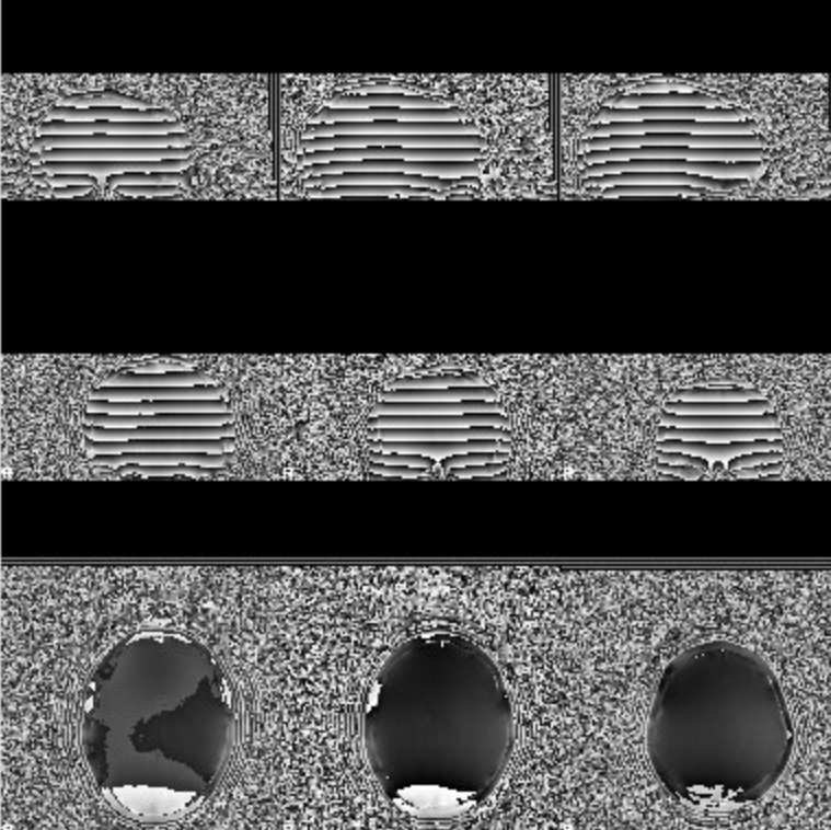
Samples of two phase maps (wrapped)
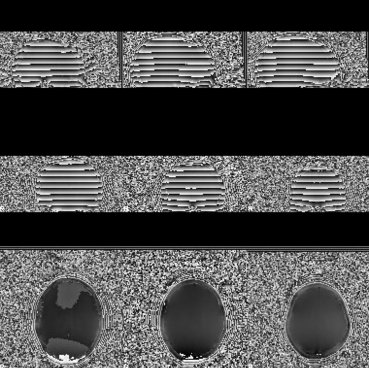
Samples of two phase maps (wrapped)
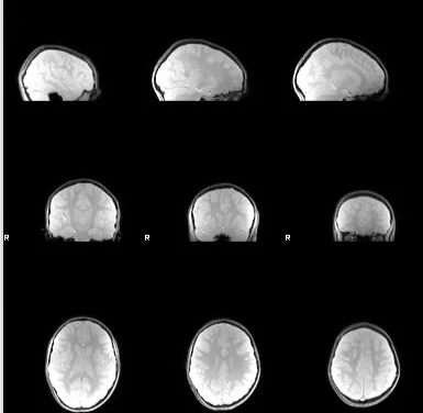
Samples of two magnitude images
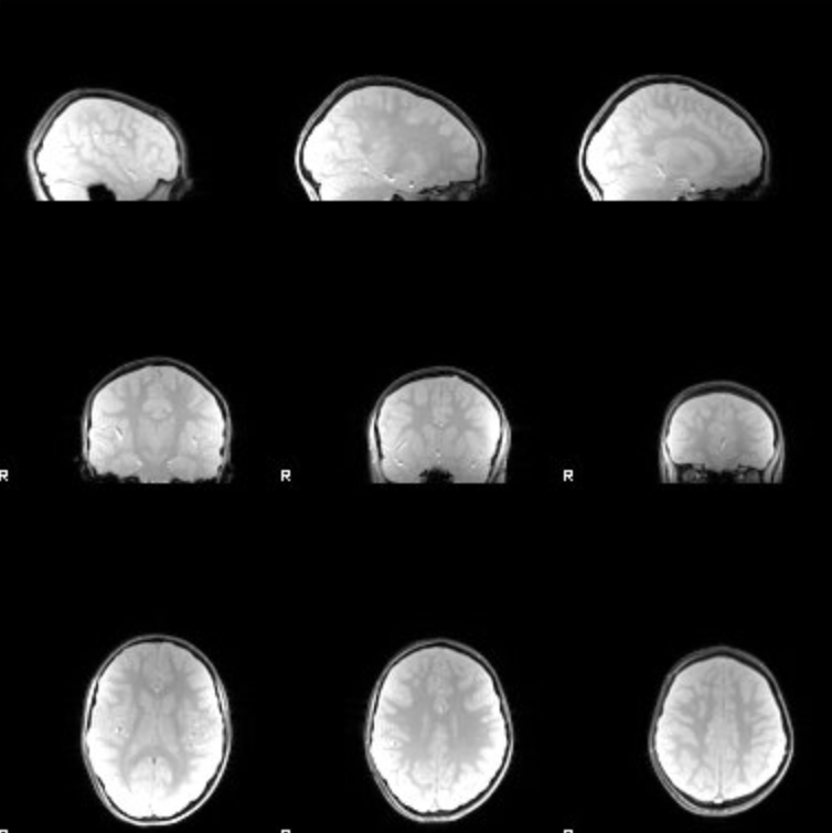
Samples of two magnitude images
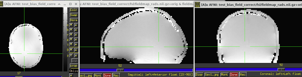
Final field map:
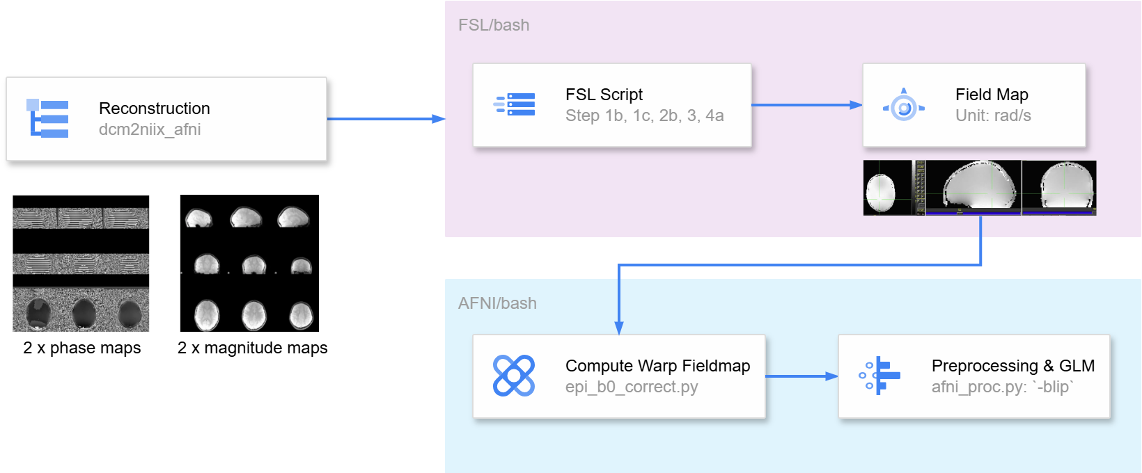
FSL + AFNI Pipeline
Based on the information provided by FUGUE “For a pair of phase images you need to do steps 1b, 1c, 2b, 3, 4a, and 5.”
Load FSL module first:
ml FSL/6.0.7.14-foss-2023a
source ${FSLDIR}/etc/fslconf/fsl.sh
Convert the DICOM files into NIFTI files. Get two phase maps and two magnitude maps.
Make sure the magnitude image and the phase maps have the same resolution by resampling (
flirt) them with a reference image (better resolution or smaller pixdims).flirt -in B*_PM1_4_ph.nii.gz -ref B*_PM1_4_.nii.gz -applyxfm -out orig_phase0 flirt -in B*_PM2_5_ph.nii.gz -ref B*_PM1_4_.nii.gz -applyxfm -out orig_phase1
Check the range first by using AFNI command
3dinfo -min -max orig_phase0.nii.gzor FSL commandfslstats orig_phase0.nii.gz -Rand found the range is [-3141, 3141]. If you usefslinfo, you will find the data_type is INT16, if your file is a complex volume, then it should be INT32. Next, usefslmathsand ensure the final range of thephase0_radimageis approximately 0 to 6.28; if not, change the value of-add,-mul, or-div`.fslmaths orig_phase0 -add 3141 -mul 3.14159 -div 3140 phase0_rad -odt float fslmaths orig_phase1 -add 3141 -mul 3.14159 -div 3140 phase1_rad -odt float
Unwrap the phase map to reduce the phase wrapping by using
prelude.prelude -a B*_PM1_4_.nii.gz -p phase0_rad -o phase0_unwrapped_rad prelude -a B*_PM1_4_.nii.gz -p phase1_rad -o phase1_unwrapped_rad
Get the final field map in rad/s by calculating the phase map difference and dividing by the TE interval. The delta TE (the difference of echo time) must be in units of milliseconds.
fslmaths phase1_unwrapped_rad -sub phase0_unwrapped_rad -mul 1000 -div 2.2 fieldmap_rads -odt float
FSL team states that “Fieldmaps can often be noisy or be contaminated around the edges of the brain. To correct for this you can regularise the fieldmap using fugue. Note that the “best” regularisation will depend on many factors in the acquisition and must be determined separately for each site/scanner/sequence. Look at the fieldmap (e.g. using fslview) to decide what is the best regularisation to use - which could also be to do no regularisation.” - for our analysis it is true that if you don’t use the following syntax, the preprocessing results will be worse, especially around the edges of the brain.
fugue --loadfmap=fieldmap_rads -s 1 --savefmap=fieldmap_radsfugue --loadfmap=fieldmap_rads --despike --savefmap=fieldmap_radsfugue --loadfmap=fieldmap_rads -m --savefmap=fieldmap_rads
In this way, we will get a field map, and then we can use the AFNI processing pipeline epi_b0_correct.py to calculate the warp field map and put it into afni_proc.py to do the preprocessing step.
AFNI’s description on the field diagram of what units to use can be a bit confusing, but the Notes section is clearly stated “It is important to have your input phase/frequency volume contain the correct units for this program. Here, we expect them to be in units of angular frequency: “radians/second” (rad/s).”
-in_epi_json: use this syntax so that you don’t need to input other parameters, such as the direction (axis) of phase encoding.in_anat: use the anatomy image as the underlay for the automatically generated QC images.do_recenter_freq MEAN: recenter the phase (=freq) volume by the mean value within the brain mask.if use
*then do not use " ", otherwise, AFNI cannot recognize it.
In the end, the script looks like this:
#!/bin/bash

echo "$1"
subj="s$(printf %03d $1)"

# Define the results directory for FSL and AFNI
fsl_results_dir="${base_dir}/${subj}/derivatives/bias_field_correct/FSL_results"
afni_results_dir="${base_dir}/${subj}/derivatives/bias_field_correct/AFNI_results"

# Create the result directories if they don't exist
mkdir -p "$fsl_results_dir"
mkdir -p "$afni_results_dir"

cd "${base_dir}/${subj}/derivatives/bias_field_correct"

# FSL pipeline, to generate a field map
flirt -in B*_PM1_4_ph.nii.gz -ref B*_PM1_4_.nii.gz -applyxfm -out "${fsl_results_dir}/orig_phase0"
flirt -in B*_PM2_5_ph.nii.gz -ref B*_PM1_4_.nii.gz -applyxfm -out "${fsl_results_dir}/orig_phase1"

fslmaths "${fsl_results_dir}/orig_phase0" -add 3141 -mul 3.14159 -div 3140 "${fsl_results_dir}/phase0_rad" -odt float
fslmaths "${fsl_results_dir}/orig_phase1" -add 3141 -mul 3.14159 -div 3140 "${fsl_results_dir}/phase1_rad" -odt float

prelude -a B*_PM1_4_.nii.gz -p "${fsl_results_dir}/phase0_rad" -o "${fsl_results_dir}/phase0_unwrapped_rad"
prelude -a B*_PM1_4_.nii.gz -p "${fsl_results_dir}/phase1_rad" -o "${fsl_results_dir}/phase1_unwrapped_rad"

fslmaths "${fsl_results_dir}/phase1_unwrapped_rad" -sub "${fsl_results_dir}/phase0_unwrapped_rad" -mul 1000 -div 2.2 "${fsl_results_dir}/fieldmap_rads" -odt float

# I used 3mm as smoothing because in the old version of fmriprep they also use this parameter: kernel_size=3
fugue --loadfmap="${fsl_results_dir}/fieldmap_rads" -s 3 --savefmap="${fsl_results_dir}/fieldmap_rads"
fugue --loadfmap="${fsl_results_dir}/fieldmap_rads" --despike --savefmap="${fsl_results_dir}/fieldmap_rads"
fugue --loadfmap="${fsl_results_dir}/fieldmap_rads" -m --savefmap="${fsl_results_dir}/fieldmap_rads"

# AFNI pipeline, you need to use the WRAP file in afni_proc.py once you finish it
# note: # if use `*`` then do not use " "
epi_b0_correct.py \
  -in_epi_json B*CEV*.json \
  -in_freq "${fsl_results_dir}/fieldmap_rads.nii.gz" \
  -in_magn B*_PM1_4_.nii.gz \
  -in_epi B*CEV*.nii.gz \
  -in_anat ${base_dir}/${subj}/derivatives/sswarp2/B*T1*nii* \
  -prefix "${afni_results_dir}/b0_corr_${subj}" \
  -do_recenter_freq MEAN
Finally, use the warp file in afni_proc.py : put the -blip_warp_dset "${base_dir}"/"s${subj}"/derivatives/kidvid_output/bias_field_correct/b0_corr_WARP.nii.gz \ between tcat_remove_first_trs and tshift_interp.
Quality Control
After completing preprocessing, you can perform qualitative quality control. Generally, alignment will be improved and geometric distortion will be reduced. Of note, distortion correction does not provide a significant improvement in data quality, and if it does, then you may need to contact a scanner engineer to improve this. It does, however, it potentially help with the alignment of EPI data and anatomy data (Reynolds et al., 2024).
Using SDC Workflow to compute fieldmap
Download singularity first:
singularity build /work/cglab/containers/sdcflows-2.10.0.sif docker://nipreps/sdcflows:2.10.0Make sure the phase and magnitude maps are in BIDS format.
Submit slurm scripts:
#!/bin/bash

# Name of the job
#SBATCH --job-name=fieldmap_sdc

# Partition on GACRC to run job
#SBATCH --partition=batch

# Number of tasks
#SBATCH --ntasks=1

# Number of compute nodes
#SBATCH --nodes=1

# Number of CPUs per task
#SBATCH --cpus-per-task=16

# Request memory
#SBATCH --mem=32G

# save logs
#SBATCH --output=/scratch/%u/workDir/log/fieldmap_sdc/fieldmap_sdc_log_array_%A-%a.out
#SBATCH --error=/scratch/%u/workDir/log/fieldmap_sdc/fieldmap_sdc_error_array_%A-%a.err

# Walltime (job duration)
#SBATCH --time=1:00:00

# Array jobs (* change the range according to # of subject; % = number of active job array tasks)
#SBATCH --array=1-3%15

participants=(174 177 191)
PARTICIPANT_LABEL=${participants[(${SLURM_ARRAY_TASK_ID} - 1)]}
BIDS_DIR=/scratch/qy49547/workDir/BIDS/
OUTPUT_DIR=/scratch/qy49547/workDir/BIDS/fieldmap_derivatives/
WORK_DIR=/scratch/qy49547/workDir/sdc_work/sub-${PARTICIPANT_LABEL}

echo "array id: " ${SLURM_ARRAY_TASK_ID}, "subject id: " ${PARTICIPANT_LABEL}

mkdir -p ${WORK_DIR}
mkdir -p ${OUTPUT_DIR}

singularity run --cleanenv \
    -B ${BIDS_DIR}:/data \
    -B ${WORK_DIR}:/work \
    -B ${OUTPUT_DIR}:/output \
    /work/cglab/containers/sdcflows-mriqc-2.10.0.sif \
    sdcflows /data /output \
    participant --participant-label ${PARTICIPANT_LABEL} \
    -w /work \
    -v --debug
You need to use WORK_DIR=/scratch/qy49547/workDir/sdc_work/sub-${PARTICIPANT_LABEL} to create separate folders, otherwise it may report erros.
Reference and Resource
https://
https://
Richard C. Reynolds, Daniel R. Glen, Gang Chen, Ziad S. Saad, Robert W. Cox, Paul A. Taylor; Processing, evaluating, and understanding FMRI data with afni_proc.py. Imaging Neuroscience 2024; 2 1–52. doi: Reynolds et al. (2024)
Hutton, C., Bork, A., Josephs, O., Deichmann, R., Ashburner, J., & Turner, R. (2002). Image Distortion Correction in fMRI: A Quantitative Evaluation. NeuroImage, 16(1), 217-240. Hutton et al. (2002)
Roopchansingh, V., French, J. J., Nielson, D. M., Reynolds, R. C., Glen, D. R., D’ Souza, P., Taylor, P. A., Cox, R. W., & Thurm, A. E. (2020). EPI Distortion Correction is Easy and Useful, and You Should Use It: A case study with toddler data. Biophysics. Roopchansingh et al. (2020)
https://
https://
https://
https://
https://
https://
https://
- Reynolds, R. C., Glen, D. R., Chen, G., Saad, Z. S., Cox, R. W., & Taylor, P. A. (2024). Processing, evaluating, and understanding FMRI data with afni_proc.py. Imaging Neuroscience, 2. 10.1162/imag_a_00347
- Hutton, C., Bork, A., Josephs, O., Deichmann, R., Ashburner, J., & Turner, R. (2002). Image Distortion Correction in fMRI: A Quantitative Evaluation. NeuroImage, 16(1), 217–240. 10.1006/nimg.2001.1054
- Roopchansingh, V., French, J. J., Nielson, D. M., Reynolds, R. C., Glen, D. R., D’ Souza, P., Taylor, P. A., Cox, R. W., & Thurm, A. E. (2020). EPI Distortion Correction is Easy and Useful, and You Should Use It: A case study with toddler data. 10.1101/2020.09.28.306787